Sequential Testing: A Practical Guide for Growth Teams

Your landing-page experiment has been running for fourteen days of a planned twenty-one. Variant B is up by 11% in conversion, the p-value is 0.04, and your product manager wants to know why you can't ship it today. The chart looks persuasive. Waiting feels wasteful.

That moment exposes the central problem in conversion-rate optimisation. A fixed-sample test assumes you'll collect the planned data, analyse it at the agreed point, and avoid making decisions based on every promising fluctuation along the way. If you repeatedly check a conventional p-value and stop when it crosses your threshold, you're no longer using the test as designed. You're giving random noise more chances to look like a winner.

Sequential testing offers a disciplined answer. It allows planned interim analysis, early stopping and continuous monitoring, provided the statistical boundaries account for every look at the data. The practical question isn't whether your team should monitor an experiment. It's how to monitor without changing the false-positive risk.

The Experiment That Would Not Stop

At the morning growth meeting, the dashboard shows a result everyone wants to believe. The new landing page has a clearer headline, a shorter form and a more direct call to action. Variant B is ahead, the confidence indicator has turned green, and the product manager is already asking engineering to prepare the rollout.

The analyst is less enthusiastic. The experiment brief specified a fixed sample size and a final analysis after the full test window. The current result has crossed the familiar p-value threshold, but the team has also looked at the dashboard throughout the test. If the original design assumed one final look, treating today's result as if it were the only analysis gives the team more opportunities to find significance than the stated method allows.

That creates an uncomfortable trade-off:

Speed: Shipping a genuine improvement earlier can free traffic for another hypothesis and reduce the opportunity cost of waiting.
False positives: Stopping after a favourable fluctuation can turn an ordinary result into a reported win.
Operational credibility: Repeatedly changing the stopping point makes experiment reports difficult to defend.
User exposure: A harmful variant should not continue running just because the calendar says the test isn't finished.

Practical rule: If stakeholders can see the result before the planned endpoint, the experiment needs a monitoring policy before launch.

The team doesn't need to choose between blind patience and impulsive shipping. It needs a stopping rule that was written before the result became exciting. That rule can define when strong evidence permits an efficacy stop, when weak evidence supports a futility stop, and how much statistical error each interim analysis is allowed to consume.

This is the day-14 question sequential testing is built to answer: how can a growth team peek responsibly without pretending that an early p-value has the same meaning as a pre-planned final analysis?

What Sequential Testing Actually Means

Sequential testing is a family of statistical procedures that analyse accumulating data at planned or continuously valid points, with a defined rule for stopping. A fixed-sample test asks you to wait for a specified amount of data and then make one principal inference. A sequential design lets evidence influence the timing of the decision, while preserving an agreed error-control framework.

A useful analogy is cooking. With a fixed-sample approach, you set a timer and taste the dish only when it rings. With a sequential approach, you check at planned stages, but you decide in advance what evidence means the dish is ready, under-seasoned, or not worth continuing. Tasting whenever you like and declaring success the first time it tastes good is something else entirely.

The language of looks and boundaries

A look is an interim analysis of the data collected so far. A stopping boundary is the threshold that the test statistic must cross before the team can stop for success, harm or futility. The null hypothesis usually represents no meaningful difference between the control and the variant.

The repeated looks matter because each analysis creates another opportunity for random variation to cross an ordinary threshold. Sequential methods adjust the decision boundaries, or use inference designed to remain valid under ongoing monitoring, so the overall Type I error probability stays controlled.

The main approaches differ in how they achieve that:

Group sequential designs schedule a defined set of interim analyses. Pocock and O'Brien-Fleming boundaries are familiar examples.
Always-valid or always-sequential methods support ongoing monitoring through procedures such as confidence sequences or sequential probability ratio methods.
Bayesian sequential approaches update a posterior distribution as observations arrive. They can express the result as a probability about which variant is better, with decision thresholds chosen by the team.

These methods aren't interchangeable. Frequentist procedures focus on controlling error rates under specified assumptions. Bayesian procedures focus on updating beliefs under a model and prior. The shared principle is more important than the label: repeated inspection must be part of the design, not an unrecorded habit.

A dashboard refresh isn't automatically wrong. A conventional p-value refreshed repeatedly without adjustment is the problem. A properly implemented sequential test turns monitoring into an explicit part of the experiment rather than an informal licence to stop whenever the chart looks favourable.

The Statistical Machinery Behind Sequential Tests

Sequential testing starts by defining the error budget. In a frequentist design, Type I error, commonly represented by alpha, is the probability of rejecting a true null hypothesis under the stated procedure. If the team sets an overall alpha of 0.05, repeated interim analyses cannot each use that full threshold as though they were separate final tests.

A group sequential design distributes that budget across planned looks. An alpha-spending function specifies how much error can be used at each stage. A Pocock-style approach usually sets more similar boundaries across looks. An O'Brien-Fleming approach sets a stricter early boundary and permits a less demanding threshold later. Each boundary defines how large the test statistic must be before the team can stop.

A two-look sketch

Consider a simplified two-look illustration with an overall alpha of 0.05, allocated as 0.03 at the first look and 0.02 at the second. These figures are educational, not a substitute for calculating a correlated group sequential boundary for a live experiment.

Design	Alpha spent per look	Critical z-value	Interpretation
Fixed-sample test	0.05 at the final analysis	Approximately 1.96 for a two-sided normal reference	One planned final decision
Sequential look one	0.03	Approximately 2.17 for a one-sided normal tail	Early evidence needs a stricter threshold
Sequential look two	0.02 in this simplified allocation	Approximately 2.05 for a one-sided normal tail	Later evidence uses the remaining budget

The exact boundary depends on whether the test is one- or two-sided, how the looks correlate, the information fraction, and the selected spending function. A simple alpha split therefore cannot replace a production-ready group sequential calculation. If alpha-spending terminology feels abstract, the CartBoss statistical significance guide explains related concepts through a worked p-value example.

Power, futility and the decision boundary

Type II error is the failure to detect a real effect. Statistical power is the complement of that error under a specified alternative. Early stopping changes the power calculation because the procedure has additional decision points and stricter early thresholds. A suitable design can preserve useful power while reducing the expected sample required when the effect is strong, but the outcome depends on the boundary, effect size, information schedule, and stopping rules.

Futility boundaries address the opposite decision. If the accumulating evidence makes the minimum effect of interest implausible, the team can stop without declaring either version a winner. That protects traffic and team attention. It also prevents a weak test from continuing just because nobody defined what “unlikely to succeed” meant before launch.

The same workflow connects clinical-trial theory with a CRO dashboard. Analysts specify the stopping rule, monitor evidence at permitted looks, and record whether the boundary was crossed. Otter A/B's continuous significance monitoring applies that principle operationally, provided the configured method accounts for ongoing inspection rather than refreshing an ordinary fixed-sample p-value.

Teams comparing frequentist and Bayesian frameworks can review this guide to the difference between Bayesian and frequentist testing. The implementation question stays concrete: what boundary was defined before observing the result, and did the current evidence cross it?

Sequential Testing Versus Fixed-Sample Designs

Fixed-sample and sequential designs solve different operational problems. A fixed-sample plan is easier to explain, calculate and audit when traffic is predictable and the decision can wait. Sequential testing earns its complexity when the team expects to monitor results, when a strong effect could justify an earlier decision, or when continuing to expose users to a poor experience carries a meaningful cost.

Dimension	Fixed-sample design	Sequential design
Decision timing	Usually one final analysis	Interim decisions are allowed
Monitoring	Analysis is tied to the endpoint	Monitoring follows planned looks or a continuously valid method
Error control	Simple when the endpoint is respected	Requires boundaries or sequentially valid inference
Sample planning	Straightforward target size	Includes stopping assumptions and often a sample-size buffer
Operations	Easy for less technical teams	More flexible, but requires documentation and tool support
Best fit	Stable timelines and patient stakeholders	High opportunity cost, safety concerns or changing conditions

The choice isn't “rigorous versus fast”. A correctly designed sequential test is rigorous in a different way. It trades some simplicity, and sometimes some fixed-sample efficiency, for the ability to act when the evidence becomes sufficiently strong.

The scenario often used in planning is a conversion rate of 4% in the control and a 6% relative lift in the variant, with an 80% power target. A fixed-sample calculation may produce a substantial visitor requirement per arm, while a Pocock-style design can permit an earlier stop when the cumulative Z-score crosses its stricter boundary. The exact sample requirement depends on the allocation, variance assumptions, look schedule and minimum effect of interest, so teams shouldn't treat a generic planning figure as a promise.

The right comparison is not “which method reaches significance first?” It's “which method gives us a defensible decision at the point where the business needs one?”

Fixed-sample testing still wins when the organisation can hold its nerve and the experiment has a clear, stable endpoint. Sequential testing is more suitable when waiting has a real opportunity cost and the team can commit to its boundaries before launch.

A Worked Example With Conversion-Rate Data

Take a simple two-arm conversion experiment. Variant A converts at 4.00% and Variant B at 4.40%, producing a raw relative lift of 10%. The test is two-tailed with alpha set at 0.05, and the team plans cumulative looks every 2,000 visitors per arm until 30,000 visitors per arm.

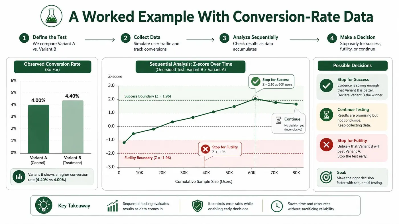
The first step is to keep the analysis cumulative. Don't compare only the latest interval, because that can mistake a temporary traffic mix change for accumulated evidence. At each look, record the visitors per arm, conversions per arm, observed rates, absolute difference, relative lift, Z-statistic, p-value and the boundary used for that look.

What the peeks appear to say

Under naive monitoring, the team might refresh a standard p-value after every look and stop at the first result below 0.05. That approach treats each interim result as though it were the only planned analysis. The apparent significance line can arrive earlier than the properly adjusted sequential boundary.

At 18,000 visitors per arm, the worked scenario has a naive p-value of 0.018, while the O'Brien-Fleming boundary still requires a p-value below roughly 0.0052 at that stage. The two methods therefore produce different operational instructions. Naive peeking says “stop”, while the pre-planned sequential rule says “continue”.

At 24,000 visitors per arm, both methods agree in the scenario. The accumulated evidence has crossed the stricter sequential boundary, so the team can make the efficacy decision under the method it selected. That agreement is useful, but it doesn't retroactively validate the earlier naive stop.

A practical recording template

For each look, write down:

Cumulative exposure, split by arm, with exclusions and data-quality checks.
Observed conversion, including the numerator and denominator rather than only a displayed percentage.
Effect estimate, with a confidence interval that matches the chosen sequential method.
Decision statistic, such as the Z-score, and the relevant boundary.
Action, stop for benefit, stop for futility, or continue.

A sample-size planning tool, such as this sample size calculator from Otter A/B, can help establish the initial fixed-horizon assumptions before the team selects a sequential design. It shouldn't replace a method-specific calculation.

The accompanying video offers another way to think about how accumulating evidence changes an experiment's decision point.

The template is defensible because it preserves the audit trail. A dashboard can show the current result, but the experiment record must show which boundary applied and why the team stopped.

How Otter A/B Handles Continuous Significance Monitoring

Continuous significance monitoring is only statistically responsible when the method accounts for repeated looks. A live p-value refreshed throughout the day isn't automatically sequential testing. Without adjustment, every refresh creates another chance for random variation to cross a conventional threshold.

Otter A/B positions continuous monitoring as an implementation of sequential thinking for web experiments. The relevant workflow is straightforward: the dashboard updates as data accumulates, but the interpretation must follow an adjusted boundary or an always-valid procedure rather than a raw fixed-horizon p-value.

What practitioners need to see

A useful monitoring view should expose more than a green badge. It should help the analyst understand:

The live confidence interval, including whether it still overlaps the minimum effect worth acting on.
The adjusted evidence trajectory, so early uncertainty isn't mistaken for final certainty.
The current boundary, showing whether the experiment has crossed the threshold for efficacy or futility.
The stop-or-continue instruction, tied to the method rather than to a stakeholder's preferred outcome.

An alpha-spending approach allocates a controlled portion of the Type I error budget to each permitted look. An always-valid method takes a different route, maintaining validity under ongoing monitoring. Either can be rigorous. Neither means every promising movement deserves a release decision.

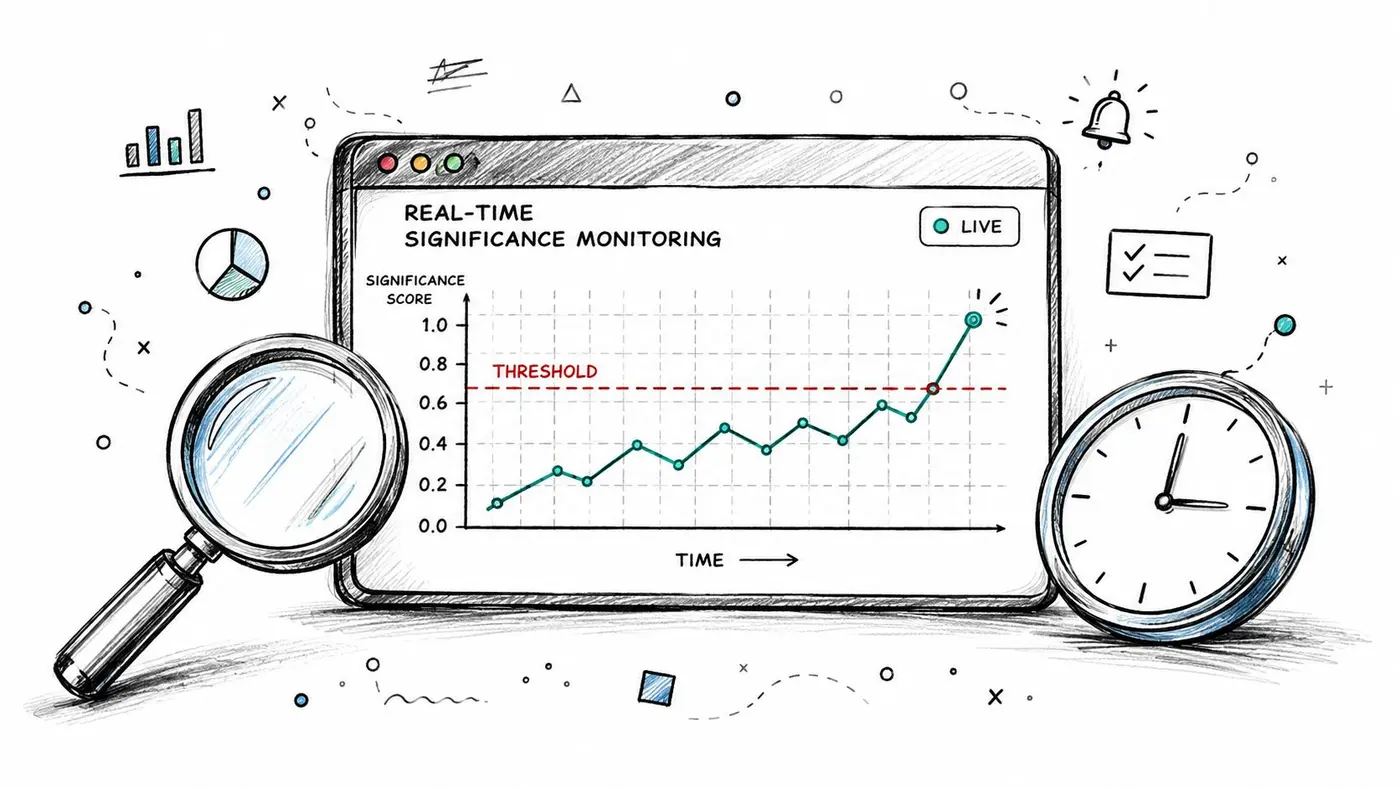
The important distinction is behavioural as much as mathematical. If the product manager checks the dashboard during a launch review, the team should already know what the displayed signal means. If the test hasn't crossed its boundary, the correct response is to continue, stop for futility if that rule has fired, or make a clearly labelled product decision outside the statistical claim.

For teams working with implementation details and integrations, Otter A/B's MCP documentation can sit alongside the experiment specification. The platform should be treated as one part of the workflow. The brief still needs to define the primary metric, monitoring method and stopping rule.

Pitfalls Every CRO Team Should Plan Around

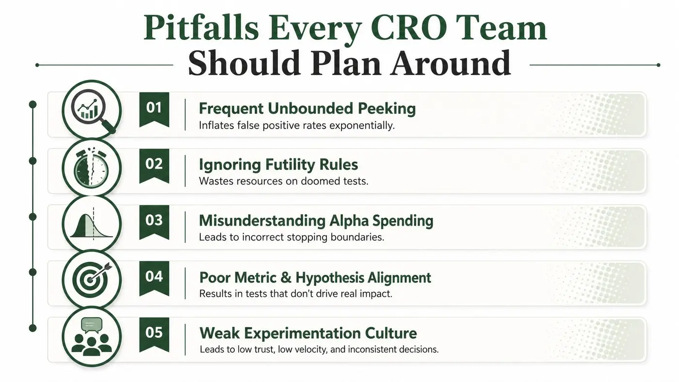
The most dangerous sequential-testing failures don't always come from difficult mathematics. They come from mismatched incentives, unclear ownership and dashboards that encourage decisions the experiment design never authorised.

Frequent unbounded peeking gives random noise repeated opportunities to look convincing. The more often a team checks an unadjusted threshold, the less meaningful the original single-look error rate becomes. A properly designed sequential test controls that problem, but only if the team uses the stated method rather than switching back to the ordinary p-value when it produces a more convenient answer.

The practical failure modes

Early winners regress: A variant can lead strongly during a short-lived traffic pattern and then move towards the underlying effect as the sample grows. Set a minimum information point and use a boundary that protects against premature efficacy calls.
Segments multiply the problem: If the team checks device, channel, geography and audience segments until one looks significant, it has created a multiple-comparisons problem. Pre-register which segments are confirmatory and treat the rest as exploratory.
Futility gets ignored: A test that cannot plausibly reach the minimum effect can consume traffic for weeks. Define a futility rule before launch, and separate “no useful effect” from “the data are still too immature”.
Urgency overrides the design: Stakeholders may still ship early because the result looks commercially obvious. Record that as a product decision, not as a statistically confirmed winner.
Sequential isn't always smaller: At equivalent power, a valid sequential design can require more planned data or a larger maximum sample than a fixed-sample design, depending on its boundaries and monitoring schedule.

Sequential testing is a discipline, not permission to peek.

The commercial context still matters. A test result only helps growth when the team connects it to a broader revenue-driven conversion strategy, including the cost of delay, implementation risk and downstream business metrics. A statistically valid stop on a narrow click metric may not justify a rollout if revenue, retention or customer quality moves in the wrong direction.

Teams should also protect the experiment from data-quality issues. Instrumentation changes, duplicate assignments, delayed conversions and uneven traffic can make a beautifully calculated boundary answer the wrong question. Statistical control can't repair a broken denominator.

Sequential Testing Checklist for Your Next Experiment

Put the decisions in the brief before traffic starts. The checklist below is deliberately operational, because sequential testing fails when its rules live only in an analyst's head.

Define the primary metric: Choose the outcome that decides the experiment and state the minimum effect of interest. Add guardrails for outcomes that could make a nominal winner unacceptable.
Choose the method: Select a group sequential design, an always-valid confidence sequence, mSPRT or a Bayesian approach based on how often the team will monitor and how it wants to express uncertainty.
Pre-register the boundary: Record the alpha-spending function, information schedule, efficacy threshold and futility rule. Don't choose Pocock or O'Brien-Fleming after seeing the trajectory.
Set the data plan: Establish the expected sample, maximum sample, allocation, review cadence and a realistic buffer. A sequential design can stop early, but it still needs enough information to detect the effect the business cares about.
Handle segments explicitly: Name confirmatory segments in advance. Treat unplanned segment findings as hypothesis generation rather than separate winners.
Align stakeholders: Explain what “continue”, “stop for benefit” and “stop for futility” mean before the first dashboard review. This prevents a product manager from negotiating with the boundary mid-test.
Validate the tooling: Confirm that the analytics system reports sequentially valid evidence, not a fixed-horizon p-value that refreshes. Check assignment, exposure, conversion windows and delayed events.
Keep the record: At every decision point, save the cumulative data, estimate, interval, boundary and action. Documentation makes the call reproducible.

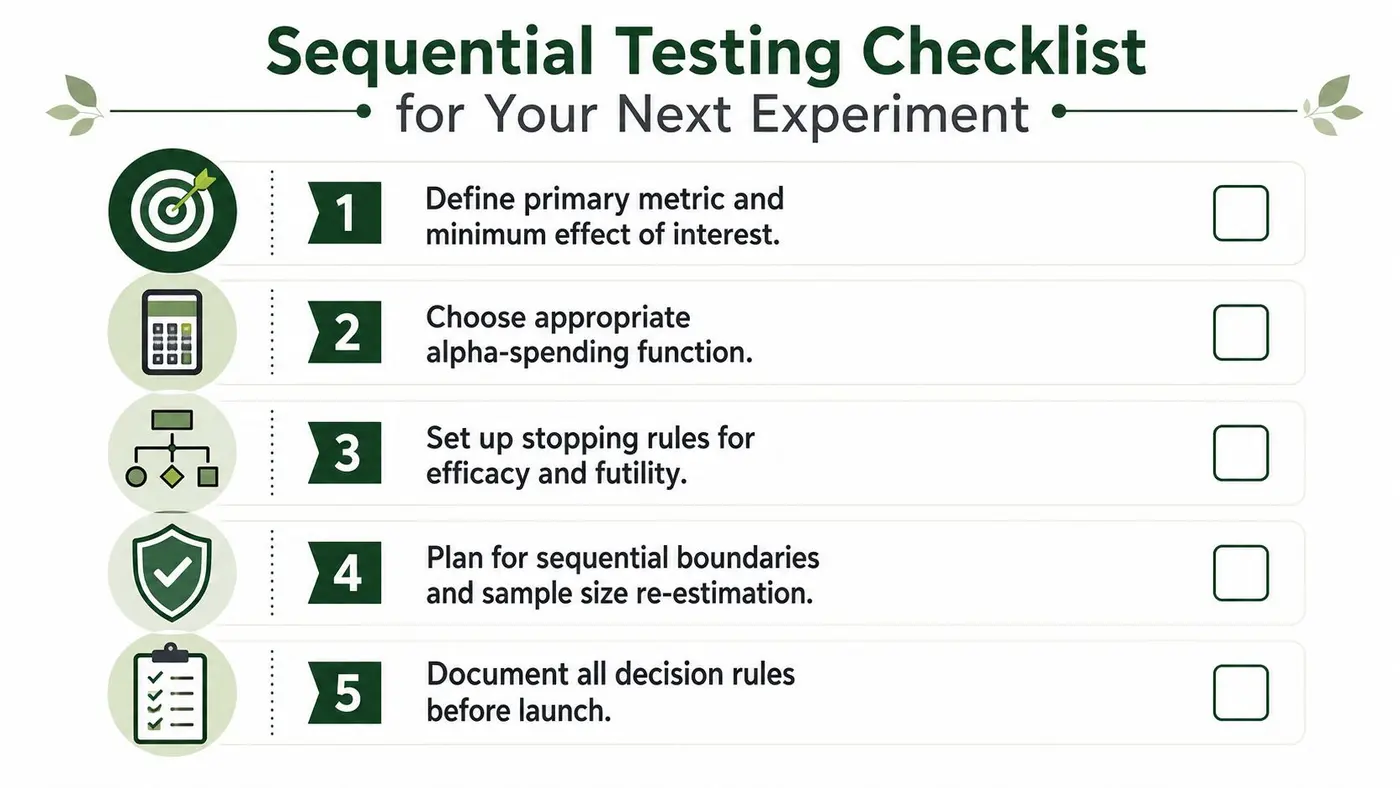
The connection between the checklist and the statistics is direct. Alpha spending protects the overall Type I error rate. Power and minimum effect planning protect the chance of finding a useful improvement. Futility rules control wasted traffic. Documentation protects the decision from hindsight.

A team that follows these steps can monitor frequently without confusing movement with evidence. It can also stop early without pretending that speed makes uncertainty disappear.

Otter A/B provides website experimentation with continuous significance monitoring, goal tracking and dashboard reporting for teams testing headlines, CTAs and layouts. Use the platform alongside a pre-written sequential testing policy, then visit Otter A/B to set up an experiment and make the next decision from an auditable evidence trail.