Ab Testing Sample Size

A marketer on a UK ecommerce team has spent three weeks watching a homepage variant climb to an apparent 22% lift. The screenshot is already in the leadership deck. By the fourth week, the result has disappeared, leaving everyone to argue whether the original uplift was insight, noise, or a change in traffic mix.

That situation is rarely caused by a bad calculator. More often, the team entered an optimistic baseline, chose an MDE because it looked attractive, launched during an unusual trading period, or stopped as soon as the dashboard looked promising. A/B testing sample size only works when the statistical plan and the operating plan agree.

Why Sample Size Makes or Breaks Your Test

Sample size is the decision that controls almost everything that follows. It determines how much traffic you commit, how long the experiment needs to run, when stakeholders can expect a decision, and whether your stopping rule has any credibility.

An under-powered test produces unstable results. A variant can appear to win because of ordinary random variation, or a useful change can fail to reach significance because the experiment didn't collect enough observations. That second outcome is especially expensive: the team may abandon an idea that could have improved performance. The opposite error ships a weak experience and exposes revenue to a false positive.

Practical rule: Treat the calculated sample as a planning requirement, not a suggestion to revisit when the dashboard looks favourable.

Sample size also differs from sample quality. A large audience won't rescue a test if tracking is broken, visitors are allocated inconsistently, or the traffic only represents a temporary promotion. A smaller sample collected across representative traffic patterns may support a better decision than a larger sample compressed into an unusual period, though neither should be judged without considering the target effect and metric.

The error trade-off is asymmetric. False positives can push a losing change into production. False negatives can stop a winning idea before the organisation has learned anything useful. An over-powered test creates a different problem, tying up traffic and development capacity after the result has already become operationally clear.

Teams working with several changing elements should also understand the extra complexity of simultaneous comparisons. Silver Spoon Agency's practical guide to multivariate testing is useful background when a proposed experiment goes beyond a straightforward control-versus-variant comparison.

Four inputs drive the calculation: the baseline conversion rate, the minimum detectable effect, the significance threshold, and statistical power. Get those inputs wrong and a precisely calculated answer can still be commercially useless.

The Four Inputs That Drive Every Calculation

Every sample-size calculator asks for the same core information, even if the labels differ. The calculation needs a trustworthy starting rate, a meaningful effect to detect, an acceptable false-positive threshold, and enough power to detect that effect when it exists.

1. Baseline conversion rate

The baseline is the current performance of the control for the metric you're testing. Use a stable, clean analytics window rather than a single recent period, because a promotion, tracking change, or unusual traffic source can distort the rate.

The baseline should match the unit and audience in the experiment. If the test allocates visitors to a product page, don't enter an account-wide conversion rate. If the primary metric is add-to-cart, don't use checkout completion as a proxy.

2. Minimum Detectable Effect

The Minimum Detectable Effect, or MDE, is the smallest improvement worth detecting and acting on. It should reflect a business threshold, not the lift the team hopes to see in a presentation.

A small relative lift can demand a very large sample, particularly when the baseline rate is low. The relationship is not intuitive, so use this MDE resource for experiment planning before entering a number into a calculator.

3. Significance level

The significance setting expresses how much false-positive risk you're prepared to accept. A 95% significance standard is a common default for higher-impact decisions, while a lower threshold may be defensible for a low-risk copy change if the team documents the trade-off clearly.

Don't choose the setting just because it produces a manageable duration. The threshold should follow the cost of being wrong.

4. Statistical power

Power is the probability that the test detects the chosen effect if that effect genuinely exists. 80% power is a conventional planning value. Higher power provides more protection against false negatives, but it also increases the traffic requirement.

Input	What it means	Typical value	Micro-example
Baseline conversion rate	Current control performance	Your observed rate	3%
MDE	Smallest commercially useful relative change	Business-defined	10%
Significance	Tolerance for false positives	95%	95%
Power	Chance of detecting the chosen real effect	80%	80%

For a worked planning combination of a 3% baseline, a 10% relative MDE, 95% significance, and 80% power, the required audience can be substantial. Treat the calculator output as a per-arm requirement, then convert it into elapsed time using real traffic. Conversion tracking also needs to reflect the business outcome you intend to improve, which is why guidance on how to optimise campaigns for your business can be useful alongside the statistical setup.

Running the Numbers With a Realistic Example

Consider a mid-market UK fashion retailer testing a new product-page layout. The primary metric is add-to-cart rate, the control baseline is 2.8%, and the team wants to detect a 15% relative lift. The plan uses 95% significance and 80% power.

The relative lift must be converted into an absolute difference before it enters a two-proportion calculation. A 15% relative increase on a 2.8% baseline produces a target variant rate of 3.22%, so the absolute effect is 0.42 percentage points.

For a two-sided two-proportion z-test, a common approximation is:

n ≈ 2p(1-p)(z_(1-α/2) + z_(1-β))² / δ²

Here, p represents the baseline proportion, δ represents the absolute difference to detect, α represents the false-positive threshold, and β represents the false-negative probability. The result is approximately 17,500 visitors per variant, or 35,000 visitors in total, for this planning scenario.

That figure is per variant, not the combined requirement. A team that mistakenly treats 17,500 as the total would finish with roughly half the planned observations in each arm and would lengthen the decision period without realising it.

Sensitivity matters more than the headline answer

The exact output changes as the baseline and MDE change. The table below is an illustrative planning view using the same 95% significance and 80% power framework. Values are rounded and intended to show the direction of the trade-off, not replace a calculator matched to your metric and test design.

Relative MDE	Baseline 2.0%	Baseline 2.8%	Baseline 4.0%	Baseline 5.0%
5%	Large requirement	Large requirement	Large requirement	Large requirement
10%	Very large requirement	Very large requirement	Very large requirement	Very large requirement
15%	High requirement	Approximately 17,500 per arm	High requirement	High requirement
20%	Lower than the 15% requirement	Lower than the 15% requirement	Lower than the 15% requirement	Lower than the 15% requirement

The calculation relationship is clear: smaller effects require sharply more observations, while higher outcome variability also increases the requirement. Experimentation literature commonly expresses that relationship as roughly 16σ²/δ² observations per arm for 95% significance and 80% power, where σ is outcome variability and δ is effect size. The formula and practical benchmark are discussed in this sample-size calculation guide.

Tools such as Evan Miller, Optimizely, and ABTestGuide can return different answers if one treats MDE as a relative lift and another treats it as an absolute percentage-point change. Check the input definition before comparing outputs. For a practical implementation, the A/B testing sample size calculator should be read as a planning aid, not as permission to stop when an early result looks attractive.

Turning Sample Size Into Test Duration

Sample size gives you the required denominator. Duration tells you how long the experiment must remain live before that denominator is reached under normal traffic.

Start with the requirement per arm, then divide the combined requirement by the page's average daily visitors when traffic is split evenly. If a test needs 20,000 visitors per arm and the page receives 1,500 visitors daily, the combined requirement is 40,000 visitors. At a 50/50 allocation, the test takes roughly 27 days, assuming traffic remains consistent.

Daily visitors to page	10,000 per variation	20,000 per variation	50,000 per variation
500	40 days	80 days	200 days
1,000	20 days	40 days	100 days
1,500	About 14 days	About 27 days	About 67 days

Those are arithmetic estimates, not launch dates. UK teams need to account for weekday and weekend behaviour, bank holidays, promotional events, and changes in consumer intent. GOV.UK guidance advises teams to use monthly visitors and expected change when deciding sample size, then run the experiment long enough to cover traffic patterns. Its guidance on sample-size planning also supports the practical principle that a test duration should reflect the size of the change being sought.

Apply operational filters

Check the launch window: Avoid starting during a major promotion unless promotional traffic is the experience you specifically want to measure.
Cover complete cycles: A test should span full weekly patterns rather than ending on a convenient weekday.
Review UK calendar effects: Bank-holiday periods can compress or redistribute traffic, so don't treat those visitors as automatically representative.
Challenge short timelines: A duration under 14 days deserves an explicit reason. Reaching the visitor target quickly doesn't prove that the traffic mix is stable.

A large sample compressed into a volatile period can still produce a misleading business decision. Conversely, spreading observations across complete traffic cycles can give the data more representative context, even when the audience arrives more slowly.

Why Peeking Breaks Your Results

A dashboard can make an unfinished test feel conclusive. On day three, the variant is ahead, the p-value briefly crosses the team's preferred threshold, and someone asks whether the result is ready for the roadmap. If the team checks repeatedly and stops at the first favourable reading, it hasn't run the test it originally planned.

Each additional look creates another opportunity to declare a winner by chance. The nominal threshold only describes the planned analysis under its planned stopping rule. Changing that rule after seeing the data increases false-positive risk, which is the central warning in guidance on sequential testing.

A result can be numerically significant and operationally untrustworthy if the team kept changing when it would stop.

Peeking isn't always reckless. Businesses sometimes need faster decisions, particularly when a test affects a time-sensitive campaign or a low-risk presentation detail. The honest trade-off is that speed can reduce decision protection unless the analysis method accounts for repeated looks.

Use a declared stopping policy

A fixed-horizon design is straightforward. Before launch, record the sample requirement, the primary metric, the significance threshold, and the earliest permitted analysis point. Then wait until the planned horizon is reached unless a serious implementation or safety issue requires intervention.

A sequential design is the disciplined alternative when the team needs to monitor results during the run. Sequential methods can reduce required traffic compared with fixed-sample designs, but they must be planned in advance. The stopping boundary, alpha-spending approach, or equivalent rule needs to exist before the dashboard starts influencing behaviour.

The practical fix is simple: make “when can we stop?” a pre-launch decision, not a debate triggered by the first attractive chart.

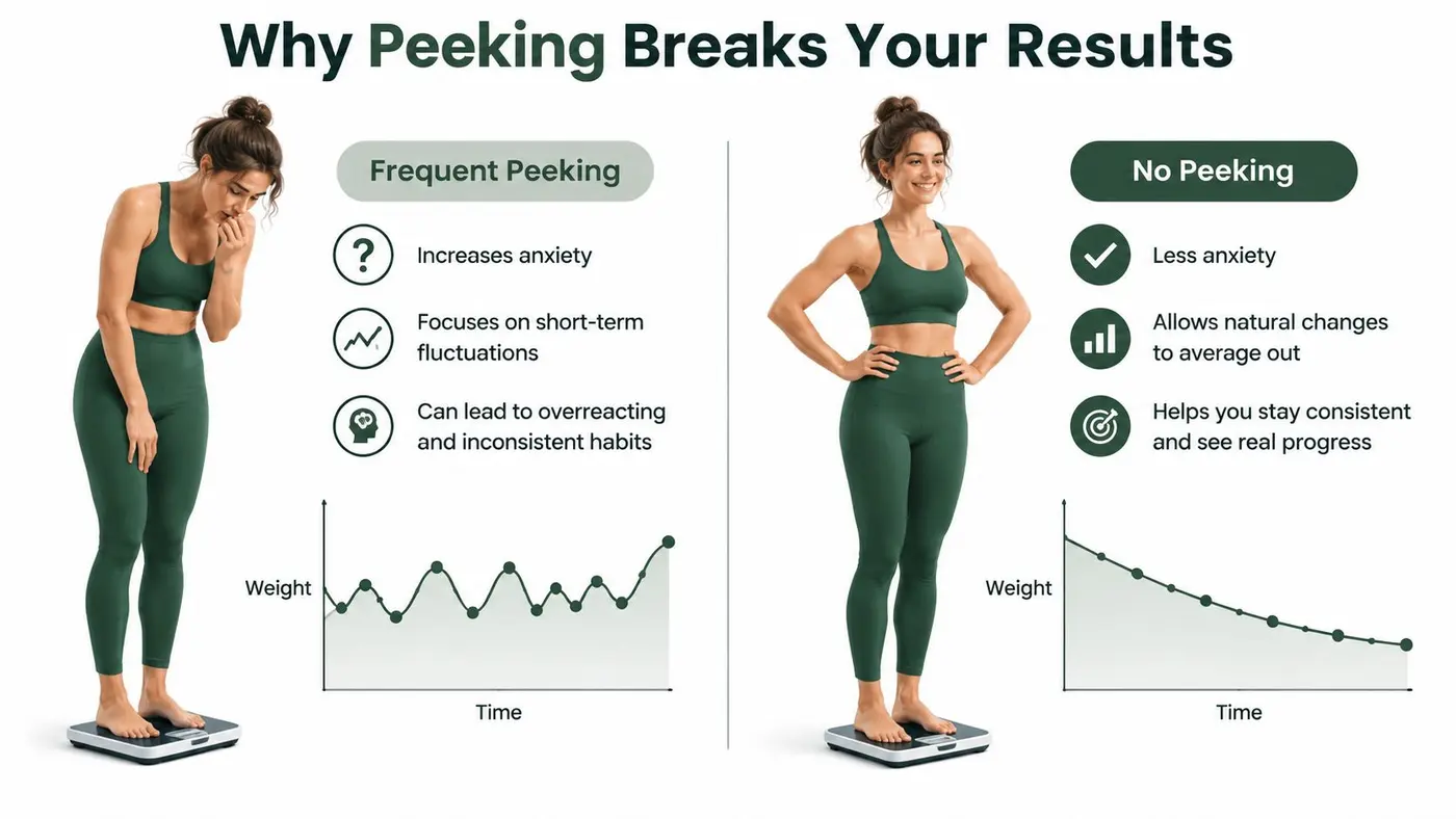
The visual above is a reminder that measurement frequency changes behaviour. In experimentation, frequent checking can turn a neutral monitoring habit into an uncontrolled stopping rule.

Use the video below as a practical companion when reviewing the difference between watching a test and making a valid decision.

Common Pitfalls and How to Dodge Them

Most sample-size failures aren't mathematical. They begin with a planning shortcut that looks reasonable under deadline pressure.

Choosing the lift you want

Teams often set the MDE at the size of the result they hope to present. That makes the test look efficient on paper, but it can leave the experiment unable to distinguish a commercially meaningful smaller improvement from noise.

Define the smallest change worth implementing. If the business wouldn't act on a modest lift, don't design the experiment to detect it. If the business would act on it, accept that the traffic requirement may be substantial.

Treating a recent baseline as truth

Last week's conversion rate may reflect a campaign, product availability, weather, or a tracking anomaly. Use a representative historical window and inspect the traffic sources, device mix, and audience eligibility before choosing the control rate.

The baseline should describe the users who will enter the experiment, not an aggregate that hides a different population.

Ending before behaviour settles

Early performance can include novelty, message priming, or an uneven distribution of returning visitors. A variant that receives attention because it's new may not retain that advantage once normal browsing behaviour resumes.

Run for the planned sample and through complete traffic cycles. If the result changes materially by weekday or audience segment, investigate before calling the experiment.

Allowing the traffic split to drift

A 50/50 test needs to receive the intended allocation. If the platform sends more users to one arm, power changes and the groups may no longer be comparable. Check the actual assignment ratio, not only the configuration screen.

Before launch, verify the experiment's allocation in observed data, not just in the tool settings.

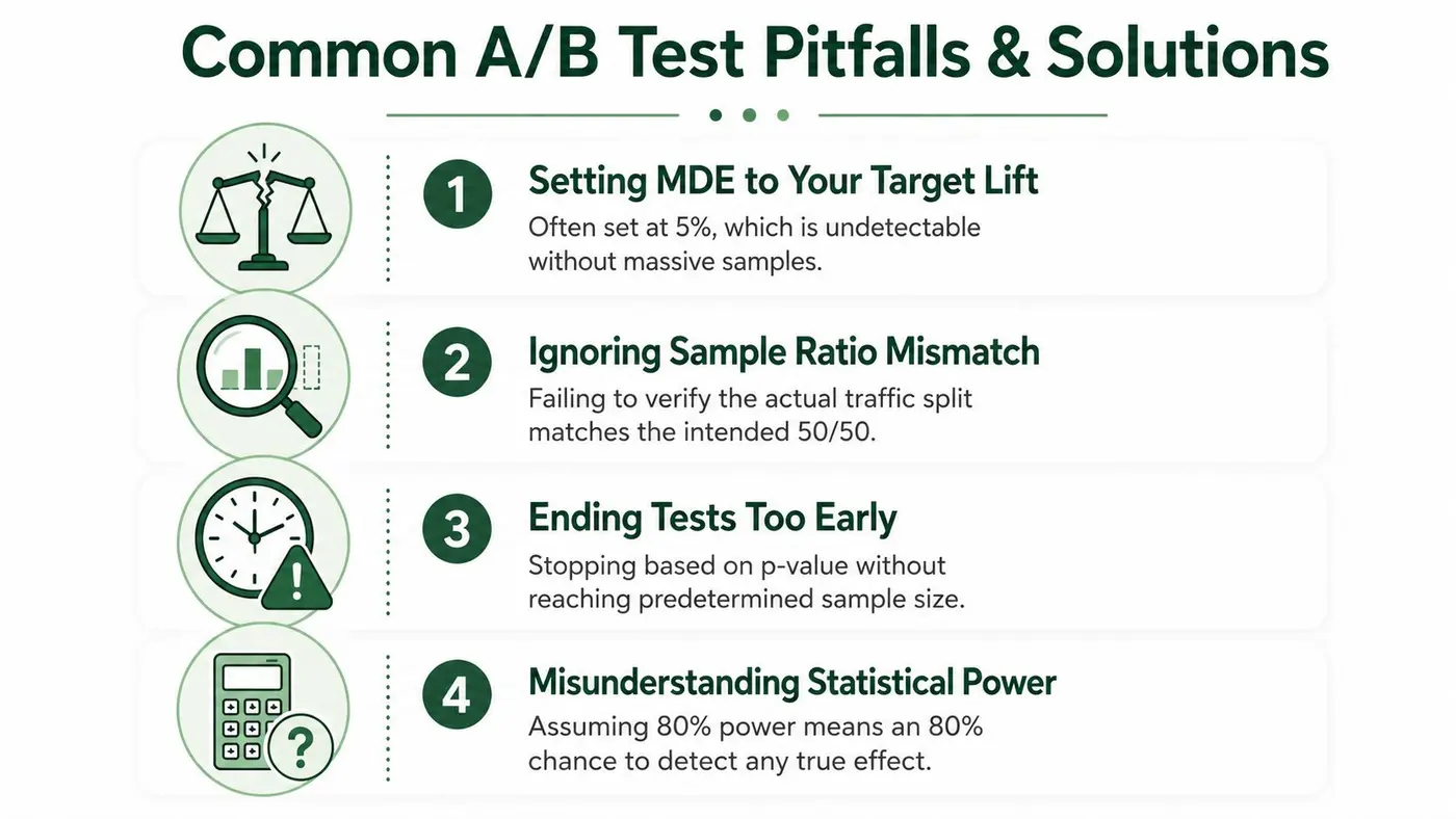
A concise pre-launch audit should record:

Baseline window: Confirm the data period and remove known anomalies.
MDE rationale: Tie the effect to a decision threshold.
Traffic allocation: Check intended and observed split.
Stopping rule: Document the sample horizon and peeking policy.
Primary metric: Name one decision metric before launch.
Calendar context: Record promotions, bank holidays, and unusual traffic conditions.

Your Sample Size Checklist Before You Launch

A reliable test plan should fit on one page. The calculation matters, but the launch decision also needs a traffic forecast, a calendar review, and a rule that prevents the dashboard from rewriting the protocol.

The five-minute sign-off

Confirm the baseline. Use clean historical data for the relevant audience and metric. Check that tracking, eligibility, and attribution are stable.
Define the MDE. Ask what minimum change would justify implementation. Record whether the calculator expects a relative lift or an absolute percentage-point difference.
Set significance and power. A practical default is 95% significance and 80% power, adjusted only when the risk of a wrong decision supports a different choice.
Calculate per-arm sample size. Write down the control and variant requirement separately, then add them to obtain the total visitor requirement.
Convert visitors into elapsed time. Use verified daily traffic, the planned split, and the expected weekday pattern. Don't treat a compressed timeline as automatically valid.
Schedule representative traffic. Include complete weekly cycles and flag promotions or UK calendar events that could change intent.
Lock the stopping policy. Decide whether the design is fixed horizon or sequential. Specify when results may be interpreted.
Log the hypothesis. State the change, audience, primary metric, MDE, sample requirement, and decision rule so another person can audit the result.

Worked launch decision

Suppose the control baseline is 3% and the team wants to detect a 10% relative lift. Enter that baseline, the relative MDE, 95% significance, and 80% power into the chosen calculator. The output becomes the per-variation visitor requirement, which the team then converts into duration using actual page traffic and checks against the UK trading calendar.

If the resulting timeline is impractical, don't shorten the test. Revisit the page, metric, audience, or MDE and make the trade-off explicit. A smaller number of variations, a higher-traffic entry point, or a more commercially meaningful effect may produce a workable plan without weakening the stopping rule.

Use this checklist before development work enters the queue. Otter A/B provides sample-size estimates within its experimentation workflow, alongside traffic allocation, goal tracking, and statistical significance reporting, so teams can connect the planning assumptions to the live test rather than relying on a disconnected spreadsheet.

Otter A/B helps teams plan and run website experiments with sample-size estimates, controlled traffic splits, goal tracking, and significance reporting for conversion and revenue outcomes. Visit Otter A/B to turn your next hypothesis into a documented test with a clear launch plan and stopping rule.