How to Calculate Confidence Interval: Step-by-Step Guide

You're staring at a test that's been live long enough for opinions to harden. Variant B is up a little, the Slack thread is getting noisy, and someone wants to ship because “the line is moving in the right direction.” A confidence interval cuts through that drift. It tells you the range of values that are still plausible for the true effect, so you can separate a real signal from the noise your sample happens to show.

Why Confidence Intervals Matter for A/B Tests

A confidence interval is the fastest way I know to answer the question teams care about, is this change real, or did we just get lucky with the sample? A single conversion rate or revenue figure looks neat in a dashboard, but it hides uncertainty. The interval puts that uncertainty back on the table in a way a point estimate never can.

In an A/B test, I use the interval around a variant's conversion rate or lift as the decision object, not the raw percentage alone. If the interval is tight, the estimate is precise. If it's wide, the test is still telling you something, just not something you should trust for a ship decision yet. For a clean primer on the underlying idea, Otter A/B has a practical explainer on what a confidence interval means in statistics.

What the 95% label actually means

A 95% confidence interval does not mean there's a 95% probability that the true value sits inside this exact interval. That's the mistake that causes the most confusion in reviews. The interval is the output of a procedure, and the 95% refers to the long-run behaviour of that procedure across repeated samples.

A better mental model is this. If you ran the same test under identical conditions over and over, about 95 out of every 100 intervals built this way would contain the true value. That's why the interval is useful in experimentation. It translates sample uncertainty into a range you can make a decision from.

Practical rule: when the team is split, the interval matters more than the headline lift. A small positive lift with a wide interval is a weak basis for shipping.

The Core Formula and What Each Piece Means

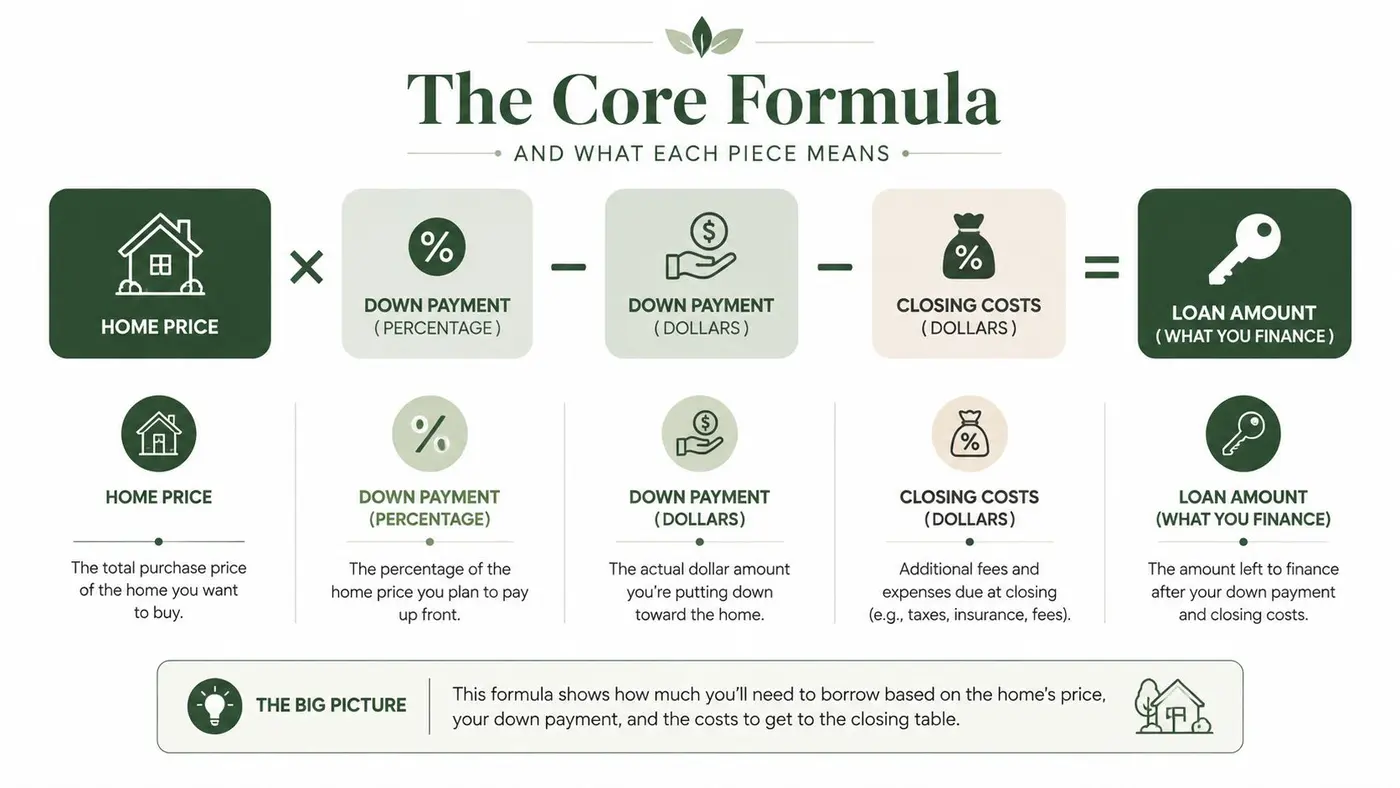
The core structure is simple, and it shows up in practical analytics and experimentation:

confidence interval = point estimate ± critical value × standard error

That formula is the one I keep coming back to in A/B tests. The point estimate is the sample result you observed, the critical value matches the confidence level you choose, and the standard error captures how much that estimate would move if you took another sample. For a practical overview of how these pieces show up in analysis workflows, the guide on practical data analysis techniques is a useful reference.

What the 95% label means

A 95% confidence interval does not mean there is a 95% probability that the true value is inside this exact interval. That wording is the source of most confusion. The interval is the result of a repeated procedure, and the 95% refers to how that procedure behaves over many samples.

The useful mental model is simpler. If you repeated the same experiment under the same conditions again and again, about 95 out of every 100 intervals built this way would contain the true value. That is why analysts use the interval to judge uncertainty, not just to report a neat-looking estimate.

Practical rule: if the team is debating whether to ship, the interval matters more than the headline lift. A small positive result with a wide interval is weak evidence for a decision.

The pieces in plain English

The standard error is not the same thing as the standard deviation. Standard deviation describes spread in the raw observations. Standard error describes how much the estimate itself would vary from sample to sample. Bigger samples usually produce narrower intervals because the estimate gets less noisy.

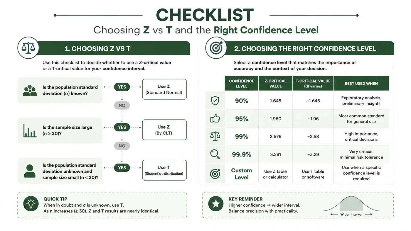
For two-sided intervals, the common critical values are easy to memorise.

Confidence Level	z-score (two-sided)	Common Use Case
90%	1.645	Faster, lower-stakes decisions
95%	1.96	Default choice for most product experiments
99%	2.576	High-stakes changes where false positives are costly

In practice, this is the part that gets used in frequentist workflows. The formula stays the same, but the width of the interval changes with the confidence level and the amount of sample noise. That is why the same lift can look convincing in one test and shaky in another.

A simple analogy helps. The interval is a net, the critical value sets how wide the net opens, and the standard error reflects how much the target is moving while you try to catch it. A wider net or a noisier target gives you a less reliable read.

Calculating a Confidence Interval for a Conversion Rate

For conversion rates, the usual starting point is the Wald interval:

p̂ ± z × √(p̂(1 - p̂) / n)

Here, p̂ is the sample conversion rate, n is the number of visitors, and z comes from your confidence level. This is a standard formula, and it's fine when traffic is healthy and the conversion rate isn't near the extremes.

A worked example

Say variant A gets 240 conversions out of 4,000 visitors. The sample conversion rate is 240 / 4,000 = 0.06, or 6.0%.

Now plug that into the standard error term:

√(0.06 × 0.94 / 4,000)

That works out to the estimated sampling spread around the rate. Multiply that by the critical value for your confidence level, then add and subtract it from 0.06 to get the lower and upper bounds. The result is the interval of plausible true conversion rates for variant A, given the sample you observed.

The Wald interval is straightforward, but it does break down when traffic is thin, the conversion rate is very close to zero, or the rate is close to one. In those cases, the Wilson score interval is a better default because it behaves more sensibly at the edges.

If you've ever worked through form abandonment rate calculation, the same principle applies, measure the rate, then put uncertainty around it before you react.

JavaScript you can copy

function confidenceIntervalForConversionRate(conversions, visitors, confidenceLevel = 0.95) {
  // Sample conversion rate, also called p-hat
  const pHat = conversions / visitors;

  // Two-sided z values for the most common confidence levels
  const zMap = {
    0.9: 1.645,
    0.95: 1.96,
    0.99: 2.576
  };

  // Fall back to 1.96 if the requested level is not in the map
  const z = zMap[confidenceLevel] || 1.96;

  // Standard error for a proportion
  const standardError = Math.sqrt((pHat * (1 - pHat)) / visitors);

  // Margin of error
  const margin = z * standardError;

  // Return the interval, bounded between 0 and 1
  return {
    lower: Math.max(0, pHat - margin),
    upper: Math.min(1, pHat + margin)
  };
}

The interval around variant A becomes your baseline. Variant B is only interesting if its interval, or the interval for the difference, gives you evidence that the lift is not just random movement.

Confidence Intervals for Means and Small Samples

For averages, the formula shifts from z to t because you usually don't know the population variance in advance. That matters most with smaller samples, which is where a lot of product teams get themselves into trouble. Average order value, time on page, and revenue per user all live here.

When the t-distribution belongs in the room

The t-distribution is the right tool when the sample is small, the population spread is unknown, or both. The shape is a little fatter in the tails than the normal curve, which is the maths way of saying it gives you a wider, more cautious interval when you don't have much evidence yet. As the sample grows, t converges towards z.

Degrees of freedom are the part people overthink. Treat them as the amount of independent information your sample still carries after you've estimated the mean. Fewer degrees of freedom means more caution, which is exactly what you want when the sample is tiny.

A Python check for average order value

import numpy as np
from scipy.stats import t

values = np.array([42, 55, 61, 38, 47, 58, 64, 41, 50, 53, 57, 44, 39, 62, 49, 46, 54, 59, 45, 52, 48, 56, 60, 43, 51])

n = len(values)
mean = values.mean()
std = values.std(ddof=1)
standard_error = std / np.sqrt(n)

confidence_level = 0.95
alpha = 1 - confidence_level
critical = t.ppf(1 - alpha / 2, df=n - 1)

margin = critical * standard_error
lower = mean - margin
upper = mean + margin

print(mean, lower, upper)

A quick rule helps in practice.

Sample size	Usual choice
Very small sample	t
Small sample with unknown variance	t
Large sample with stable variance	z or t, usually similar
Mixed or uneven variance between groups	Welch's t approach

If you want a deeper reference for z-based workflows, Otter A/B has a direct guide on the z test in statistics.

Choosing z vs t and the Right Confidence Level

This choice is less about ceremony and more about the shape of your decision. For a single proportion, z is the common starting point. For a mean with unknown variance, t is safer. For a difference between variants, the sample structure matters too, because independent groups and paired measurements do not behave the same way.

How I choose confidence levels in experiments

The confidence level sets how much false-positive risk you're willing to tolerate in exchange for narrower or wider intervals. 95% is the safe default in most experimentation programmes because it balances caution and usability. 99% belongs on changes where a bad call is expensive. 90% can make sense when speed matters and the downside of a false positive is low.

A decent practical guide on t test examples for business helps when your metric is a mean and you need to decide whether the extra caution from t is worth it. That's the point, don't treat z versus t as a religion. Treat it as a decision about how much uncertainty you have.

In an A/B workflow, Otter A/B uses a 95% confidence threshold for its frequentist significance engine, which is a sensible default for product teams that want a clear ship or hold decision. That default is not magic, it just aligns with the level many teams are already comfortable using.

Margin of Error and Required Sample Size

The margin of error is just the half-width of the interval. For a proportion, the algebra is direct:

MOE = z × √(p(1 - p) / n)

Rearrange it and you get the sample size formula:

n = z² × p(1 - p) / MOE²

That's the planning equation teams use when they want to know whether a test can answer the question they care about.

A planning example

Suppose your baseline conversion rate is 4%, and you want to detect a 5% relative lift. That means the target difference is small, because 5% of 4% is only a slight increase in absolute terms. At 95% confidence, the z critical value is the usual 1.96.

If you plug the baseline rate into the formula and choose a tight margin of error, the required sample gets large quickly. That's why many tests look “promising” early and then flatten out later. The signal you wanted was never strong enough to support an early stop.

Python to estimate visitors per variant

import math
from scipy.stats import norm

def required_sample_size(baseline_rate, min_detectable_effect, confidence_level=0.95, power=0.8):
    # Convert relative lift into an absolute lift
    absolute_effect = baseline_rate * min_detectable_effect
    target_rate = baseline_rate + absolute_effect

    # Two-sided z critical value for confidence
    alpha = 1 - confidence_level
    z_alpha = norm.ppf(1 - alpha / 2)

    # Z value for desired power
    z_beta = norm.ppf(power)

    # Pooled proportion approximation
    p_bar = (baseline_rate + target_rate) / 2

    numerator = (z_alpha * math.sqrt(2 * p_bar * (1 - p_bar)) + z_beta * math.sqrt(
        baseline_rate * (1 - baseline_rate) + target_rate * (1 - target_rate)
    )) ** 2

    denominator = absolute_effect ** 2

    return math.ceil(numerator / denominator)

The important operational point is simple. Per-variant traffic split and continuous significance calculations only help after the test has enough data to support them. Before that, you're looking at instability, not evidence. Peeking early makes the nominal false-positive rate meaningless.

For a fuller planning walkthrough, Otter A/B also has a focused guide on how to calculate sample size.

Reading the Interval to Call a Winner in A/B Testing

The rule is cleaner than most dashboards make it look. If you're testing the difference between two variants, a 95% confidence interval for the lift that stays entirely above zero means B is beating A with statistical support. If it stays entirely below zero, A is better. If it crosses zero, the test is still inconclusive.

That statement is mathematically equivalent to saying the two-sided p-value is below 0.05 when the interval excludes zero. Teams often treat those as separate ideas, but they're the same decision criterion expressed in different language. One is easier to explain to stakeholders, the other is easier to calculate in code.

How to read the result without overthinking it

The positive or negative sign matters first. The width matters second. A narrow interval that sits above zero is usually actionable. A wide one that barely clears zero deserves caution, especially if the business impact is small.

Don't ship a winner just because the line moved. Ship when the interval, the effect size, and the guardrails all line up.

Otter A/B surfaces this sort of decision with a frequentist engine that calculates significance continuously at the 95% threshold, and it sends Slack notifications when a winner emerges. It also keeps the rest of the business in view by tracking things like revenue per variant, average order value, and revenue trends over time, so you don't end up promoting a higher-converting page that harms revenue. If you need to share the outcome with clients or stakeholders, the brandable, password-protected reports are useful because they keep the result tied to the experiment rather than to a screenshot in a slide deck.

The five mistakes that break interpretation

1. Peeking too early. Checking daily and stopping the moment significance appears inflates false positives. Pre-commit the sample size, or use sequential methods.
2. Treating the interval like a probability about the parameter. It isn't. The interval comes from a repeatable procedure, not a one-off probability statement.
3. Assuming overlapping intervals mean no difference. That shortcut fails often. Test the difference directly.
4. Ignoring imbalance in variance or sample size. Uneven groups need the right variance handling, often Welch's t approach.
5. Reporting the interval without business context. Pair it with absolute lift, revenue impact, and segment behaviour, or the number won't tell you enough.

The cleanest takeaway is the one experienced teams keep relearning. An interval is only as useful as the assumptions behind it.

---

If you want a workflow that turns confidence intervals into actual ship-or-hold decisions, explore Otter A/B. It pairs frequentist significance with revenue tracking, Slack alerts, and client-ready reporting, so you can see when an experiment is done and move on with less debate.